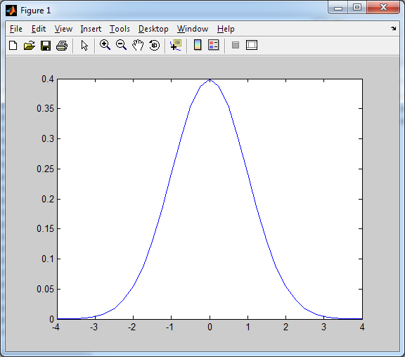
Gaussian noise is another type of noise commonly encountered in image processing. It gets this name because the noise spectrum (ie: a histogram of just the image noise over a blank background) has a Gaussian/normal distribution, as shown below.
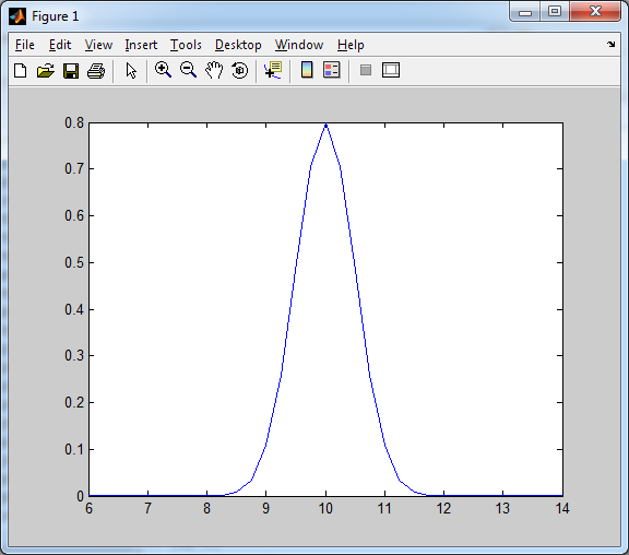
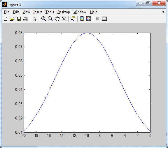
A normalized Gaussian distribution has a mean (average) value of zero (0), and a variance (spread) of one (1). The mean essentially points out where the peak of the curve is with respect to the x-axis, and the variance tells us how wide or spread-out the values are from this point. Consider the curves below, where we play around with the variance and mean of a normalized curve.
Notice how the peak is at the mean value (10), and the smaller variance has caused the curve to be compressed in the horizontal axis (less spread).
Now consider the example above. The curve’s peak is centered at the mean (-10), while the increased variance has caused the curve to spread-out more along the x-axis.
Now, with respect to image processing, the addition of Gaussian noise essentially means that the input image has been altered due to the addition of a Gaussian random variable with mean and variances
, where
is the square-root of the variance, also known as the standard deviation. So, for each pixel in the original source image, the output after the addition of noise will be roughly equal to the sum of the original pixel value, and a random variable in the neighborhood of the mean value of the noise being added.
Before we continue, we should ask ourselves this: how can we generate Gaussian noise to apply to an image. MATLAB comes with a tool, normpdf, which allows us to generate a Gaussian/normal distribution easily enough, but we’d prefer to do everything from the ground-up so that we can learn more from this. One method for generating a Gaussian distribution with a mean of zero (0) and a variance of one (1) is the Box-Muller method as described in [1].
First, consider two random variables, and
, both of which are independent random variables on [0,1]. We can generate from these values, two separate random variables which will approximately fall within a random distribution with a mean of zero (0) and a variance of one (1), by using the following formulae:
Once we’ve generated enough Z-values using these formulae (using different random values for and
each time, of course), the Z-values will roughly approximate a normalized Gaussian/normal distribution, according to the central limit theorem [2]. Now, we’d like to be able to change the mean and variance of this distribution so that we can experiment with Gaussian distributions other than just the normalized Gaussian distribution (ie: something other than just mean = 0, variance = 1).
This is actually a very simple operation, since we already have a normalized Gaussian distribution. If we add a constant to each Z-value we generated, we effectively change the mean by the constant. As for the variance, if we multiple each Z-value by a constant, the variance increases by the square of that constant. So if we want to take a normalized Gaussian distribution (mean = 0, variance = 1), and we’d like to change the mean to , and the variance to
, we simply perform the following operation on each Z-value we generated previously:
A MATLAB function for generating ‘nVals’ data points that form a Gaussian distribution with a mean of ‘meanVal’ and a variance of ‘varVal’ is shown below, demonstrating how I have implemented this approach to creating arbitrary Gaussian distributions.
%==========================================================================
function output_data = genNormDist(meanVal, varVal, nVals)
%   genNormDist     -   Generates a normal/Gaussian distribution with mean
%                       of 'meanVal', variance of 'varVal', and 'nVals'
%                       discrete values in the distribution.
%                       This method uses the Box-Muller method to create an
%                       approximation to a normal distribution with mean of
%                       '0' and a variance of '1'. The data set is then
%                       multiplied by sqrt(varVal) to change the variance
%                       to 'varVal', and then has meanVal added to each
%                       term to adjust the mean, respectively
%   output_data     -   The processed data
%   meanVal         -   The mean
%   varVal          -   The variance
%   nVals           -   The number of values in the distribution
% (C) 2010 Matthew Giassa, <teo@giassa.net> www.giassa.net
%==========================================================================
%Make sure variance isn't zero
if(varVal <= 0)
 error('Can not proceed: Variance cannot equal zero or be negative!')
end

%Create a data buffer
tempVector = zeros(1,nVals);

%Use the Box-Muller method to generate pairs of random variables, and
%store them in the tempVector buffer
for counter = 1:2:nVals
 %Generate two random variables on [0,1]
 U1=rand(1);
 U2=rand(1);
 %Calculate our Z-values
 Z0=sqrt(-2*log(U1))*cos(2*pi*U2);
 Z1=sqrt(-2*log(U2))*cos(2*pi*U1);
 tempVector(counter) = Z0;
 tempVector(counter+1) = Z1;
end

%Adjust the mean and variance
tempVector = tempVector.*sqrt(varVal) + meanVal;

%==========================================================================
% Completed
%==========================================================================
output_data = tempVector;
Now that we have a method for generating a normal distribution, we can apply Gaussian noise to an image by simply “adding” the distribution to the original source image. One simple approach to this is to generate a Gaussian distribution with a specific mean and variance, and the number of elements should be equal to the number of pixels in the source image. Then, simply randomize the order of the individual values in the distribution, and add it as an array to the image buffer. The sample code below demonstrates this in action.
%==========================================================================
function output_image = addGaussianNoise(input_image, meanNoise, varNoise )
%   addGaussianNoise -  Adds Gaussian noise to an image
%   output_image    -   The processed image
%   input_image     -   The source image data
% (C) 2010 Matthew Giassa, <teo@giassa.net> www.giassa.net
%==========================================================================
%Make a grayscale copy of our input image
I = double(rgb2gray(input_image));

%Determine input image dimensions
[j k] = size(I);

%Create a Gaussian random variable distribution
randVals = genNormDist(meanNoise, varNoise, j.*k);
size(randVals)
%Reshape the image
I = reshape(I,1,[]);
size(I)
%Add the Gaussian noise
I = I + randVals;
mean(I)
var(I)

%Revert the image back from a 1D vector to a 2D image
I = reshape(I,j,k);

%==========================================================================
% Completed
%==========================================================================
output_image = I;
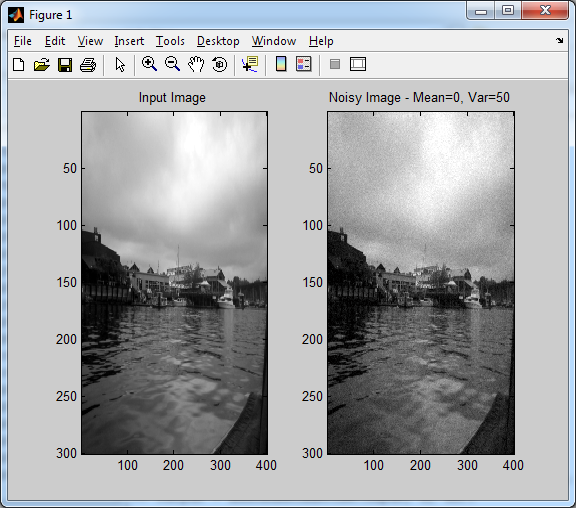
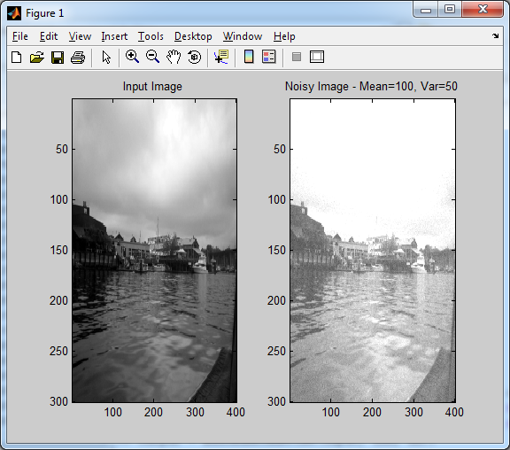
A few sample images are provided below with different means and variances assigned to them using the code above. It should give you a visual representation of how changing these parameters will affect the final result.
In case you haven’t guessed it by now, changing the mean will change the average brightness of the image, while increasing the variance will make the image more noisy (ie: the random “speckles” everywhere become more noticeable).
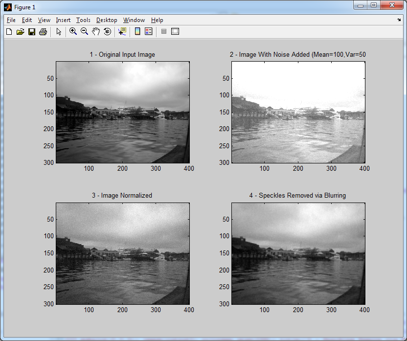
Now that we’ve learned what Gaussian noise is with respect to image processing, along with a means of generating it in arbitrary amounts, we need a way to remove it. Fortunately, we already know how! We know from the earlier section on image normalization that we can deal with changes to the average brightness of an image simply by normalizing it. That takes care of the new mean intensity value. As for the “speckles”, we can remove those by blurring the image with a simple convolution masks. The code for these algorithms can be found in previous sections of these tutorials, so they will not be reproduced here. An example run-through of this process is shown below.
You will notice that the input image and the final result are not identical. You could theoretically use varying sizes of convolution masks for blurring the noisy image in the final step, and calculate separate error vectors for each case to see which one yields the smallest error value. In most cases, a convolution mask larger than 5×5 will generally tend to blur the image too much and decrease the quality of the output. As is the case in practically any engineering problem, there are always trade-offs. In this case, how much noise can we remove without decreasing the output image quality too much.
References
[1] “Box-Muller Transformation — from Wolfram MathWorld.” Wolfram MathWorld: The Web’s Most Extensive Mathematics Resource. Web. 26 Apr. 2010. <http://mathworld.wolfram.com/Box-MullerTransformation.html>.
[2] “Central Limit Theorem — from Wolfram MathWorld.” Wolfram MathWorld: The Web’s Most Extensive Mathematics Resource. Web. 26 Apr. 2010. <http://mathworld.wolfram.com/CentralLimitTheorem.html>.


Wicked. Nice that someone actually does all the algorithms from scratch for creating AND fixing the noise.
When are you doing the stuff on floodfill? A 3d one would be useful.
I’ll be doing the 2D seedfill algorithm within a month, 2 tops.
The 3D version is VERY easy to create from the 2D one. Also, I have some simple demo apps that show 2D cross-sections of a 3D “image” and let you click on them to change their color. Kind like MS paint in 3D (or at least part of it).
it is very useful for me. Thank you so much !