Not even two months before I completed my work designing an interface for the impedance analyzer used at the SFU Microinstrumentation Laboratory, I jumped on board with a project involving SFU and BC Cancer Agency, utilizing an impedance analysis system as a possible cancer screenin system. Taking the impedance analyzer, a small netbook, my existing interface system, and additional tools we developed, we have…

System Overview Diagram

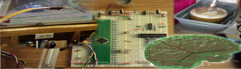
Actual System

With this system, we used breast phantoms composed of gelatin and saline solution, along with an electrode array with a stationary electrode placed in the center of the phantom, and multiple selectable electrodes along the circumference of the phantom, as outlined below.

Inital Electrode Placements

Using this electrode array, we could generate Cole-Cole plots between electrode ‘A’ and the remaining electrodes. In the case where a small amount of lipid, calcium, and salt was placed between two electrodes (to mimic a potential breast tumor), we were able to consistenly generate Cole-Cole plots with different parameters compared to samples that had no such anomaly injected. These changes were most prounounced at lower frequencies between five to six kiloHertz (kHz).

Cole-Cole Plot

One downfall to the existing system was that the electrode placement at the time only allowed for detection of foreign substances in the breast phantom that were close to the surface, indicated by the orange regions in the “Initial Electrode Placements” diagram above. We could generate basic impedance maps that show a general region where the lipid/calcium deposit was injected, but not with enough accuracy.

Simple Impedance Map (Upper Left) and Interpolated Impedance Map (Lower Right)

We changed our electrode placement to that shown below.

new electrode placement

Combined with a more sophisticated  EIT image reconstruction software we designed over the course of several months (please refer to “Publications” section), we were able to generate 2D impedance maps of the breast phantom, indicating the location of the injected lipid/calcium deposit. Although the error bounds for the size of the anomaly injected into the phantom are large, the centroid is located with a reasonable degree of accurary.

2D Image Reconstructed from our EIT Software

We are now at the point where we are preparing to improve on this system, possibly allowing for us to extend our image reconstruction system to provide a fully 3D impedance map, indicating the precise location of the injected lipid/calcium deposit. This may demonstrate the viability of impedance analysis as a non-invasive, low-cost, and rapid means to screen for breast cancer in its early stages.

3D Extrapolation from 2D Image