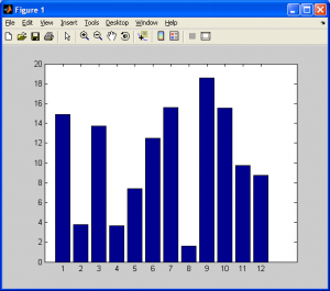
A histogram is a simple type of bar chart that indicates the total number of occurences of a certain condition across multiple categories. A simple example would be calculating the number of of inches of rain per month over an entire year in Vancouver, BC, as demonstrated below (note that these ARE NOT actual statistics, they are simply made up).
So, the vertical axis indicates how much rain there was per month, and the horizontal axis indicates the month. Nothing too complex here. Now, when we extend this to image processing, we are doing the exact same thing, except we are now interested in calculating the number of pixels with specific intensity values. Consider a grayscale image, with 256 different possible intensity values such that:
- Zero (0) represents a black pixel.
- The largest value (255) represents a white pixel.
- All integer values between 0 and 255 represent shades of gray.
- The closer to 0, the darker the shade of gray, and the closer to 255, the lighter the shade.
- Note that we can arbitrarily define a larger range of gray values, such as 0 to 65535, but for simplicity, I’ll keep it on the range of [0,255] for now.
- Also note that these ranges are almost always a “power of two minus one”. More on this later.
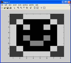
Now, consider a simple tiny image, like the one shown below of a smiley face.
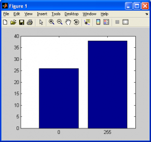
So, for each pixel value, we need to make a tally (ie: a running sum) for each intensity value in the source image. As we can see from the image above, this is an 8×8 pixel black-and-white image, amounting to a total of pixels total. Based on the rules above, we should have a simple histogram with values for 0 and 255 only, and the totals for each “bar” in our histogram should add up to 64. We can create a histogram for this by hand just by counting the total number of black pixels (intensity value of 0) and white pixels (intensity value of 255). For the above image, I calculated a total of 26 black pixels and 38 white pixels. Sure enough,
pixels, so that should rule out any errors such as counting a pixel twice. The histogram is shown below:
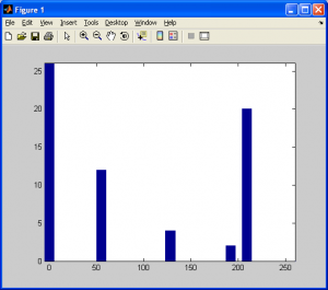
Now, consider an image with several different gray values on the interval [0,255], as shown below:
The corresponding histogram is included below:
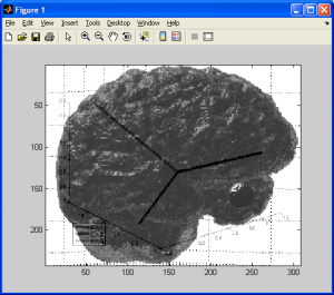
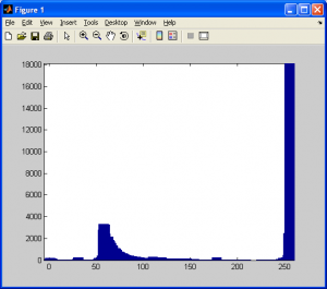
As you may have already guessed, for larger images with more data, we’ll have more bars present in the histogram. The final example below provides histogram data for a sample MRI image.
Next, I will present a simple MATLAB M-function for generating a histogram for a grayscale image. The HIST and IMHIST functions in MATLAB can do this easily enough, but it’s more fun to do this from scratch. Note that, assuming all pixel intensity values are discrete integer values, we can easily generate a histogram quickly by using the pixel intensity value as the histogram array’s index variables, as demonstrated below. The results can be displayed by executing “bar(ImageHist(I))”, where “I” is a 2D image data array.
function hist_matrix = ImageHist( input_image )
%Generates and displays a histogram for an input image after first
%converting it to grayscale
%INPUT_IMAGE    -   The input image data to process
%==========================================================================
%Import a copy of the original image data and convert it to grayscale
I=rgb2gray(input_image);
%Determine the dimensions of the input image
[j k] = size(I);
%Calculate the maximum and minimum intensity values in the original image
min_val = min(min(I));
max_val = max(max(I));
%Declare the histogram matrix which will store the tallied values
hist_data = zeros(1,double(max_val)+1);
%Although the original image may contain an intensity value of zero, MATLAB
%arrays and vectors begin addresses with one rather than zero. Take note of
%this.
for counter1 = 1:j
 for counter2 = 1:k
 index_val = 1+double(I(counter1,counter2));
 hist_data(1,index_val) = hist_data(1,index_val)+1;
 end
end
hist_matrix = zeros(2,double(max_val)+1);
hist_matrix(1,:)=0:1:max_val;
hist_matrix(2,:)=hist_data(1,:);
%Done
Now that we know how to generate histogram data, we’ll take a look at some statistics that can help us gain more insight into the significance of a histogram with respect to image processing. First, consider the mean (ie: “average”) intensity value of all of the pixels in the image. We can think of this as the average brightness of the entire image. A low mean would mean that most of the image is relatively dark, while a high mean would mean that the majority of the image is quite bright.
We can calculate the mean by summing up the intensity values of all the pixels in the source image, then dividing by the total number of pixels. NOTE: If you ever attempt this algorithm for an important project, consider reading up on numerical analysis and the the problem of adding small numbers to large numbers. It is possible to add a very small number to a very large number, and the sum is simply the larger of the two numbers. I’ll leave it to the reader to look into this issue, as it is more a programming issue in general with which the reader should be familiar.
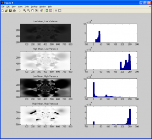
With the mean pixel value available to us, we should also consider calculating the variance, the square-root of which is the standard deviation. This effectively tells us the “spread” of pixel intensity values about the mean value. A low variance indicates that most of the pixel intensity values are very close to each other (ie: a picture of pavement – most of the image is gray, with a few dark spots, possibly due to shadows). A high variance would indicate a lot of “spread” about the mean value. Consider a picture of pavement with some dark spots due to oil or dirt, and some very bright spots due to reflections. The following images, along with their histograms, should help to provide more insight into this concept before we conclude this subsection. Notice how a high variance causes the histogram to span over a larger range, while a lower variance confines it to a smaller range, as well as how the mean essentially defines the “midpoint” of the histogram.

