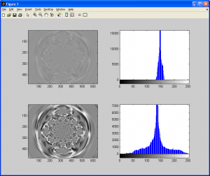
If you took a careful look at the previous subsection on histograms, you may have noticed that the narrower the histogram of an image is (ie: less variance in the histogram spectrum), the less contrast an image has. I’ll give another example below of an image with very low variance (poor contrast), and the same image with a contrast adjustment algorithm applied to it:
In both cases, the original images have the same number of pixels, but the histogram for the second image with contrast enhancement applied to it has a much wider histogram (ie: greater variance/standard-deviation). There are several different ways to alter an image to improve contrast, but I will only cover one of them for now. I leave it up to the reader to use these guides to devise your own original methods for contrast enhancement.
First, consider a gray-scale image with 256 different possible intensity values on the range [0,255]. As mentioned in the previous subsection, most of the time, when dealing with images, intensity values are stored as discrete numbers (ie: integers) rather than floating point numbers (which have a fractional component). Due to the internal workings of computers in general, we generally store numbers as binary values. Common limits for the maximum size of an integer could be 255 for an 8-bit unsigned number (), 65535 for a 16-bit unsigned number (
) and so on. In the case of the examples I have been discussing so far, I have been converting color images to 8-bit gray-scale images to make the tutorials simpler. As I also mentioned in the first section in this tutorial, there is an easy way to extend all of these algorithms to deal with color images, not just gray-scale ones.
Anyhow, the images we are working with can have an intensity value between 0 and 255 (inclusive) assigned to each pixel. Let’s assume the image we are working with has poor contrast, and after histogram analysis, we realize that, for ALL of the pixels in the source image, the intensity values are on a sub-interval, [a,b], such that and
(An example would be that the smallest intensity value is 17, and the largest is 40. That would imply that
and
).
We want to scale and shift all of the intensity values in our source image so that we can recreate the original image with all of the intensity values reassigned to an appropriate value on [0,255]. One very simple approach to this is the following “single pixel operation” (ie: each pixel in the output image is a function of a single pixel in the source/input image. In this case, we calculate some statistics from the source image and perform a linear shifting/scaling operation on the pixels in the source image to generate the pixels in the output image):
- Define the upper and lower limits for intensity values in the final output image (
and
; we are assuming that
, as we want the output histogram to be on the interval
)
- Determine the upper and lower limits for intensity values in the source image, either by a simple search algorithm or histogram analysis (
and
)
- “Shift” all of the intensity values by subtracting the value
from each of them
- “Scale” all of the intensity values by multiplying them by
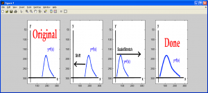
The following figures demonstrate the equivalent operation for a 1D data set:
This particular type of contrast adjustment can also be referred to as image normalization, because it normalizes the intensity values of the source image over the entire available data range (ie: [0,255]). The following MATLAB M-function demonstrates how one may implement this algorithm. More importantly, pay attention to how it makes use of the intmax(‘uint8’) and intmin(‘uint8’) code to determine the upper and lower limits for an unsigned 8-bit integer rather than using a sentinel value hard-coded into the program. This type of approach should always be taken as it will save you headaches and hours of debugging down the road. Similar functions exist in C/C++, or your can design them yourself with relative ease (refer to [1]).
%==========================================================================
function output_image = imnorm( input_image )
%   IMNORM  -   Normalizes image intensity values over [0,255]
%   output_image    -   The normalized image
%   input_image     -   The source image data
% (C) 2010 Matthew Giassa, <teo@giassa.net> www.giassa.net
%==========================================================================
%Make a grayscale copy of our input image
I = double(rgb2gray(input_image));
%Determine input image dimensions
[j k] = size(I);
%Determine the extreme intensity values for our input image
in_min = double(min(min(I)));
in_max = double(max(max(I)));
%Determine the extreme intensity values for the output image
out_min = double(intmin('uint8'));
out_max = double(intmax('uint8'));
%Determine the amount to "shift/move" pixel intensity values by
shift_val = in_min - out_min;
%Determine the value to "scale" pixel intensity values by
scale_val = (out_max)/(in_max-in_min);
%Perform the shift and scale (in that order)
for counter1 = 1:j
 for counter2 = 1:k
 I(counter1,counter2)=(I(counter1,counter2)-double(shift_val))*double(scale_val);
 end
end
%Done
output_image = I;
One important concept to consider when implementing this algorithm is avoiding clipping. Consider a gray-scale image that may have pixel intensity values on the internal [0,255]. Now, let’s say you attempt to implement a normalization algorithm that normalizes pixels on a larger interval, say, [0, 65535], but the data type you are using to represent a pixel can only hold a maximum value of 255. In the end, your image looks terrible, and a disproportionately large number of pixels are white (ie: set to 255). This is because of several pixels being saturated (ie: reaching their maximum possible value; adding more doesn’t change anything). This effect is known as clipping.
Depending on the data structure you use to represent a pixel, you can encounter clipping, or, if you are unlucky enough, overflow for individual pixels values. This occurs when a pixel value is already at its maximum possible value, and attempting to increase this value causes the pixel value to roll over to either zero or a negative number, creating seemingly random pixel values. Although I would expect it to be a prerequisite to the topic of image processing, anyone who intends to take part in this subject should seriously consider studying the basics of numerical analysis as well so that avoiding issues like these becomes a habit.
References
[1] Prata, Stephen. C Primer Plus (5th Edition). Indianapolis: Sams, 2004. Print.


