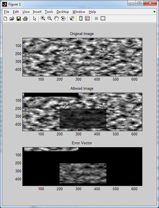
To conclude this section of the tutorial, I decided to save the best for last – error vectors. A more appropriate term would be an error matrix, but we’ll let it slide in this case, since the concept is can be explained in terms of either of the two.

Let’s say you have an input image, , and you want to carry out an operation on it, , such that:

Now let’s assume that you are attempting to recreate the the original function using a different algorithm. We will call this new function . So, theoretically, if was implemented properly, both functions should yield the same output. We’ll assume that this is not the case, and that, due to an error in our code somewhere, the two functions do not produce identical output for the same input image, . We will define the output of our experimental function, , as:

Once we’ve calculated the test and control output images, we can compare them pixel-by-pixel to see if they produce the same output. This seems like an obvious technique, and some might wonder why I would bother putting it up here. An important note to remember is that some algorithms, especially iterative ones, do not generate the same output each time, even if the input data does not change between runs.

So, it would be nice if we could somehow have some sort of simple statistic to tell us “how different” our control and test images are. A simple and effective approach is to simply take the absolute value of the difference of the two images, store it in an image buffer itself, then calculate the sum of all pixel values. This value, the “error value”, can be used to assess how consistent your results are across runs.

I should also mention that for larger images, the error value can become very large. Make sure your error value doesn’t saturate or roll over!

Image, Altered Image, and Error Vector

%==========================================================================
function output_image = errorVector( input_image )
%   output_image    -   The normalized image
%   input_image     -   The source image data
% (C) 2010 Matthew Giassa, <teo@giassa.net> www.giassa.net
%==========================================================================
%Make a grayscale copy of our input image
I = double(rgb2gray(input_image));

%Determine input image dimensions
[j k] = size(I);

%Determine the extreme intensity values for our input image
in_min = double(min(min(I)));
in_max = double(max(max(I)));

%Determine the extreme intensity values for the output image
out_min = double(intmin('uint8'));
out_max = double(intmax('uint8'));

%Determine the amount to "shift/move" pixel intensity values by
shift_val = in_min - out_min;

%Determine the value to "scale" pixel intensity values by
scale_val = (out_max)/(in_max-in_min);

%Perform the shift and scale (in that order)
for counter1 = 1:j
 for counter2 = 1:k
 I(counter1,counter2)=(I(counter1,counter2)-double(shift_val))*double(scale_val);
 end
end

%At this point we've simply normalized an input image - nothing new here.
%However, we can now make a copy of this normalized image, perform a few
%random operations on it, and then compare the two
I2 = I;

%Set a few pixels to zero (0)
I2(5:50,10:300) = 0;
%Now make a few a lot darker
I2(200:450,200:450) = I2(200:450,200:450)./3;

%Generate plots
subplot(3,1,1); image(I); colormap gray(255); title 'Original Image';
subplot(3,1,2); image(I2); colormap gray(255); title 'Altered Image';

error_value = sum(sum(abs(I-I2)));
subplot(3,1,3); image(abs(I-I2)); colormap gray(255); title 'Error Vector';
disp(sprintf('The sum of all pixel values in the error vector is %f',error_value))

%Done
output_image = I;