If you haven’t read the previous section on bicubic spline interpolation, now would be a good time!
As mentioned in the previous section, when we are performing bicubic interpolation, we are generating a smooth surface that interpolates data points on a 2D grid. Also, as previously mentioned…
Quote:
So, we can see that we have taken the original data set, and interpolated values in both the x and y dimensions to create a smooth surface. An important note: Notice how the interpolated dataset is smooth in the x-direction, y-direction, and the xy-direction (ie: along the diagonals). This means that for any point in our interpolated data set, we should be able to compute not only the intensity (ie: height/grayscale) value, but also it’s derivative in ANY direction along x, y, or xy. This is equivalent to us having the following data available to us (assume the grayscale intensity value from the source image,
, at
, and that we are trying to calculate the interpolated grayscale value in the target/output image,
, at
) (Equations based on those provided in [1]):
- The original intensity values of the surrounding pixels (4 values)
- The partial derivatives along the x-axis for each of these points (4 values)
- The partial derivatives along the y-axis for each of these points (4 values)
- The cross-derivatives at each of these points (4 values)
This leaves us with a total of 16 values to solve for in the case of generalized bicubic interpolation, as opposed to the 4 needed with 1D cubic spline interpolation ( and
).
End Quote
I also mentioned in the previous section that bicubic spline interpolation is a special case of generalized bicubic interpolation. For the former of the two, we simply carried out 1D cubic spline interpolation along each axis and we were done. We aren’t making use of all the data available to us though, such as the cross-derivatives.
For each of the neighbouring 4 data points, we need to know its intensity value (), its partial derivatives along both axes (
and
), and finally, its cross-derivatives (
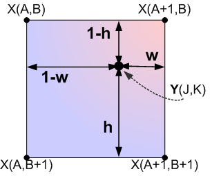
) before we can proceed any further. Before we proceed these, we need a coordinate system, as always. Notice how we now need to know the values of (1-h),(1-w), etc, whereas when we carried out bicubic spline interpolation we didn’t!
We can calculate the partial derivatives easily enough using centered differences, which are basically slope calculations using the intensity values, from adjacent pixels. For the partial derivative along the horizontal axis,
, we can calculate it to be (assuming equal spacing between pixels in the source image):
Similarly, we calculate the partial derivative for the vertical axis at each neighbouring pixel by:
Finally, for the cross derivatives, we can calculate them by:
- Therefore,
If the spacing between pixels is not equal (ie: you are only carrying out interpolation on part of an image rather than the whole thing), you will need to adjust the denominator values in the above equations. Note that even if you get these values wrong, the final result will still be smooth, just not as accurate!
With these values available, we can defined any interpolated value in our output/target image, , as a function of the pixels from our input image according to (refer to the grid coordinates in the figure above for visual definitions of A,B,J,K,h, and w):
However, before we can carry on, we need to solve for the coefficients, . Assuming that
and
are continuous over the interval
, and that we redefine the values at the gridpoints of the source image,
as
, we can express all 16 coefficients of
as follows (equations provided by [1]):
- Function values:
- X-Derivatives:
- Y-Derivatives:
- Cross-Derivatives (XY):
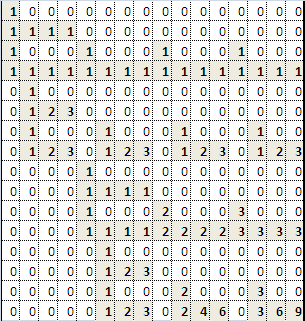
These coefficient values, combined with the previously calculated partial and cross-derivative values, form a set of linear equations which form a matrix equation of the general form . We will rewrite it in the form
so that we don’t confuse the values for our matrices with those used in the equations above. Let:
Note that the refers to the transpose of these matrices, rather than an exponent (which would only make sense for a square matrix anyways). With these equations, we can use our favorite method (feel free to pick) of solving this set of linear equations to solve for the inverse of our weighting matrix,
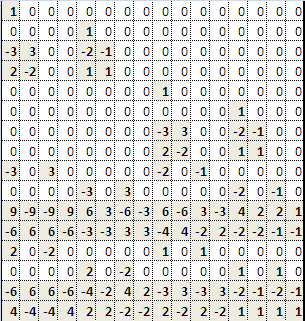
. Once this is done, we can save this matrix for use in any future implementations of bicubic interpolation, as there is no need to recalculate it again in the future. By simple matrix inversion (yes, you can do this by hand if you really want to, the matrix algebra is very simple, just time-consuming; it’d be better to do this with MATLAB), we get the inverted coefficient matrix,
.
=
When is multiplied (via matrix multiplication of course) with our product matrix,
, this gives us the values of each of the 16 coefficients in our
matrix. We can now use the previously defined sigma-notation formula to determine the value of any interpolated data point using the formula:
The following MATLAB M-function demonstrates this algorithm in action:
% GBI.M
% Written December 2009, (C) Matthew Giassa
% teo@giassa.net, www.giassa.net
% Returns an upsampled image using bicubic interpolation
function output_image = gbi( input_image,x_res,y_res )
%   input_image     -   an image on which to perform bicubic interpolation
%   x_res           -   the new horizontal dimensions (in pixels)
%   y_res           -   the new vertical dimensions (in pixels)
%Define the inverted weighting matrix, M^(-1), no need to recalculate it
%ever again
M_inv = [
 1,0,0,0,0,0,0,0,0,0,0,0,0,0,0,0;
 0,0,0,0,1,0,0,0,0,0,0,0,0,0,0,0;
 -3,3,0,0,-2,-1,0,0,0,0,0,0,0,0,0,0;
 2,-2,0,0,1,1,0,0,0,0,0,0,0,0,0,0;
 0,0,0,0,0,0,0,0,1,0,0,0,0,0,0,0;
 0,0,0,0,0,0,0,0,0,0,0,0,1,0,0,0;
 0,0,0,0,0,0,0,0,-3,3,0,0,-2,-1,0,0;
 0,0,0,0,0,0,0,0,2,-2,0,0,1,1,0,0;
 -3,0,3,0,0,0,0,0,-2,0,-1,0,0,0,0,0;
 0,0,0,0,-3,0,3,0,0,0,0,0,-2,0,-1,0;
 9,-9,-9,9,6,3,-6,-3,6,-6,3,-3,4,2,2,1;
 -6,6,6,-6,-3,-3,3,3,-4,4,-2,2,-2,-2,-1,-1;
 2,0,-2,0,0,0,0,0,1,0,1,0,0,0,0,0;
 0,0,0,0,2,0,-2,0,0,0,0,0,1,0,1,0;
 -6,6,6,-6,-4,-2,4,2,-3,3,-3,3,-2,-1,-2,-1;
 4,-4,-4,4,2,2,-2,-2,2,-2,2,-2,1,1,1,1
 ];
%Make a copy of the input image
I = input_image;
%Convert image to grayscale (intensity) values for simplicity (for now)
I = double(rgb2gray(I));
%Determine the dimensions of the source image
%Note that we will have three values - width, height, and the number
%of color vectors, 3
[j k] = size(I);
%Specify the new image dimensions we want for our larger output image
x_new = x_res;
y_new = y_res;
%Determine the ratio of the old dimensions compared to the new dimensions
%Referred to as S1 and S2 in my tutorial
x_scale = x_new./(j-1);
y_scale = y_new./(k-1);
%Declare and initialize an output image buffer
temp_image = zeros(x_new,y_new);
%Calculate the horizontal derivatives for each point (assume that at the
%edge pixels of the source image, all derivatives are zero to maximize
%smoothing). Take note - recreating this in C or C++ might not be so easy,
%as you must pay attention to how this code is using matrix-style
%addressing (x-y positions swapped).
Ix = double(zeros(j,k));
for count1 = 1:j
 for count2 = 1:k
 if( (count2==1) || (count2==k) )
 Ix(count1,count2)=0;
 else
 Ix(count1,count2)=(0.5).*(I(count1,count2+1)-I(count1,count2-1));
 end
 end
end
%Similarly, calculate the vertical derivatives
Iy = double(zeros(j,k));
for count1 = 1:j
 for count2 = 1:k
 if( (count1==1) || (count1==j) )
 Iy(count1,count2)=0;
 else
 Iy(count1,count2)=(0.5).*(I(count1+1,count2)-I(count1-1,count2));
 end
 end
end
%Finally, calculate the cross derivatives
Ixy = double(zeros(j,k));
for count1 = 1:j
 for count2 = 1:k
 if( (count1==1) || (count1==j) || (count2==1) || (count2==k) )
 Ixy(count1,count2)=0;
 else
 Ixy(count1,count2)=(0.25).*((I(count1+1,count2+1)+I(count1-1,count2-1)) - (I(count1+1,count2-1)+I(count1-1,count2+1)));
 end
 end
end
%Generate the output image
%==========================================================================
%Please note that this is definitely not the most efficient way to carry
%out this operation, as we are recalculating our beta and alpha-vectors far
%repeatedly when there is no need. I kept the code like this so you can see
%the order in which we would carry out most operations. If you want to make
%a more efficient version which pre-calculates the alpha vector for each
%pixel in the source image, be my guest.
%==========================================================================
for count1 = 0:x_new-1
 for count2 = 0:y_new-1
 %Calculate the normalized distance constants, h and w
 W = -(((count1./x_scale)-floor(count1./x_scale))-1);
 H = -(((count2./y_scale)-floor(count2./y_scale))-1);
 %Determine the indexes/address of the 4 neighbouring pixels from
 %the source data/image
 I11_index = [1+floor(count1./x_scale),1+floor(count2./y_scale)];
 I21_index = [1+floor(count1./x_scale),1+ceil(count2./y_scale)];
 I12_index = [1+ceil(count1./x_scale),1+floor(count2./y_scale)];
 I22_index = [1+ceil(count1./x_scale),1+ceil(count2./y_scale)];
 %Calculate the four nearest function values
 I11 = I(I11_index(1),I11_index(2));
 I21 = I(I21_index(1),I21_index(2));
 I12 = I(I12_index(1),I12_index(2));
 I22 = I(I22_index(1),I22_index(2));
 %Calculate the four nearest horizontal derivatives
 Ix11 = Ix(I11_index(1),I11_index(2));
 Ix21 = Ix(I21_index(1),I21_index(2));
 Ix12 = Ix(I12_index(1),I12_index(2));
 Ix22 = Ix(I22_index(1),I22_index(2));
 %Calculate the four nearest vertical derivatives
 Iy11 = Iy(I11_index(1),I11_index(2));
 Iy21 = Iy(I21_index(1),I21_index(2));
 Iy12 = Iy(I12_index(1),I12_index(2));
 Iy22 = Iy(I22_index(1),I22_index(2));
 %Calculate the four nearest cross derivatives
 Ixy11 = Ixy(I11_index(1),I11_index(2));
 Ixy21 = Ixy(I21_index(1),I21_index(2));
 Ixy12 = Ixy(I12_index(1),I12_index(2));
 Ixy22 = Ixy(I22_index(1),I22_index(2));
 %Create our beta-vector
 beta = [I11 I21 I12 I22 Ix11 Ix21 Ix12 Ix22 Iy11 Iy21 Iy12 Iy22 Ixy11 Ixy21 Ixy12 Ixy22];
 %Calculate our alpha vector (ie: the a-values) using simple matrix
 %multiplication
 %==================================================================
 %If we wanted to make sure this entire program is written entirely
 %from scratch, we would implement our own code to multiple an AxB
 %matrix and a BxC matrix right here. This is very simple to do, so
 %I won't go over it right now.
 %==================================================================
 alpha = M_inv*beta';
 temp_p=0;
 for count3 = 1:16
 w_temp = floor((count3-1)/4);
 h_temp = mod(count3-1,4);
 %disp(sprintf('aij=%d  wsub=%d   hsub=%d\n',count3,w_temp,h_temp))
 temp_p = temp_p + alpha(count3).*((1-W)^(w_temp)).*((1-H)^(h_temp));
 end
 temp_image(count1+1,count2+1)=temp_p;
 end
end
output_image = temp_image;
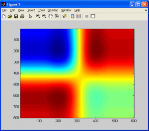
Included below is a simple resampling of a 4×4 checkerboard pattern to a much larger resolution using the code above.
Before concluding this section, I should note that there are many other resampling methods that are definitely worth reading up on, such as Lanczos, Hermite spline, Super Eagle, 2xSAI, HQn, and so on. Many of these algorithms are used in commerical products such as image processing software digital cameras, even console emulators. I will now conclude this section with a brief comparison of “bicubic spline interpolation” and “generalized bicubic interpolation”, and will show why the two are NOT the same.
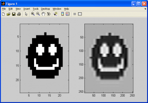
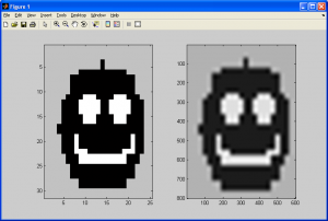
First, observe the image pairs below. The first pair was generated by using bicubic spline interpolation, which was covered in the previous subsection, while the latter pair was generated with the generalized bicubic interpolation algorithm covered in this subsection (the two original smiley faces used are slightly different, but no matter):
If we observe the resampling smiley faces, we can see that both still have halos introduced due to our choice of resampling algorithms. One important difference exists between both of the sampled images, however – the former of the two (generated using bicubic spline interpolation) still demonstrates some sharp edges and even corners, while the latter does not. This is due to bicubic spline interpolation being a rough approximation of generalized bicubic interpolation at best, primarily due to it not making any use of the cross-derivatives of the source data.
References
[1] Numerical recipes in C the art of scientific computing. Cambridge: Cambridge UP, 1992. Print.

