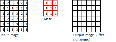
As mentioned at the beginning of this section, the use of spatial convolution masks is a straightforward extension of discrete convolution to two (2) dimensions. A simple example is demonstrated below. First, consider the following three objects:
- An input image, whose dimensions must be equal or greater than those of the mask (described below)
- A convolution “mask” (usually it is a square matrix, and its dimensions are odd; ie: 3, 5, 7, etc)
- An output image buffer which is the same size as the input image
The actual mathematics behind this operation is rather simple and straightforward. First, lets imagine that we “stack” the mask on top of the input image so that the upper-left corners of both the mask and the input image are touching. Now, for each pixel where the mask “overlaps” the input image, calculate the product of the value in the “mask pixel”, and the the “image pixel”, and sum these up (in the above example, assuming we are going from left-to-right, then top-to bottom, the calculation would be: ). We then take this sum-of-products, find the “centre” pixel of where the mask overlaps with the input image, and put the sum in the output image buffer at the same “centre” pixel location, as shown below.
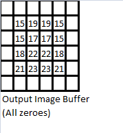
We then repeat “slide” the mask from left-to-right, then top to bottom, so that we’ve carried this operation out on every pixel for which the mask can overlap the input image without leaving the boundaries of the input image. The next few iterations of this operation are shown below to demonstrate this operation in action.
Proceeding in this manner, we eventually arrive at the convolution sum output which we stored in the output image buffer, as shown below.
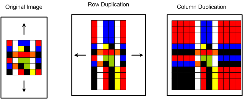
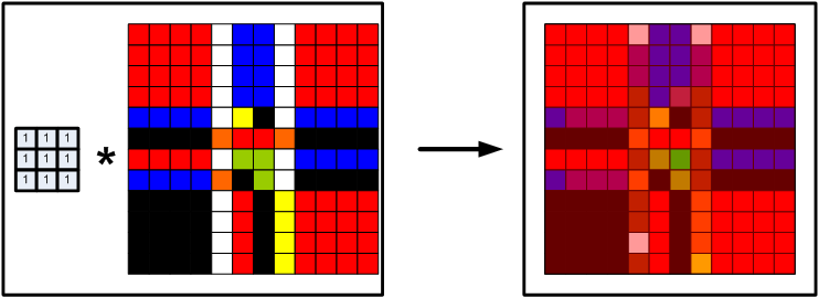
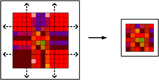
There is still a problem with this operation though – the border pixels are all zeroes! In image processing, this is the equivalent of having a black border in the output image. What’s worse is that if we were to use a larger mask (say, 5×5, or 11×11), or perform multiple convolution operations on an image, we would have a very small output image. We could always “trim” the image to remove these borders, but the output image will become smaller each time we do this. There must be a reasonable workaround, and there is. One simple enough method is to simply replicate the columns of the input image, then the rows, carry out convolution, then “trim” the output image, as shown below.
So, consider an input image with dimensions by
, and a convolution mask with dimensions
by
, such that
(ie: it is a square matrix with odd dimensions). Therefore, the number of columns on both the right and left-hand-side of the input image that need to be replicated are
. Once we have replicated columns on the left and right, the same number of rows need to be replicated on the top and bottom of the input image. From there, we simply perform the convolution of the input image, and then trim
rows/columns from the top, bottom, left, and right of the final output image buffer. This will result in a better output image that also has the same dimensions as the original input image. The following MATLAB code below demonstrates this concept in action, and can be used to test any arbitrary mask. Please note that it also normalizes the images, but this feature can be removed easily enough. Enjoy!
%==========================================================================
function[A] = imgMask(src_matrix,mask_matrix)
% imgMask   Applies a variable sized image mask to an image
% src_matrix is the original image to copy and modify afterwards
% mask_matrix is the coefficient matrix to use

% Copy original image data to a temporary buffer
% and flatten to a 2D grayscale matrix
copy_matrix = src_matrix;
copy_matrix = squeeze(copy_matrix(:,:,1));

% Determine the dimensions of the source matrix
[x,y] = size(copy_matrix);

% Determine the dimesnions of the mask matrix
[a,b] = size(mask_matrix);

% Error checking code
% Non-square mask matrix
if(a~=b)
 disp(sprintf('Mask matrix is not square!'))
elsif((a==0) | (b==0))
 disp(sprintf('Mask matrix has a singleton dimension!'))
elsif((a<3) | (b<3))
 disp(sprintf('Mask matrix is not at least 3x3!'))
elsif((a>=(x-1)) | (b>=(y-1)))
 disp(sprintf('Mask matrix dimenions are too large!'))
else
 % Calculate sum of values in mask matrix
 scaler = double(sum(sum(mask_matrix)));
 if(scaler == 0)
 %disp(sprintf('Mask matrix has a net sum of zero!\n'))
 end
 % Pad the matrix edges so we don't lose data
 for j = 1:b
 [a_temp, b_temp] = size(copy_matrix);
 copy_matrix = vertcat(copy_matrix, copy_matrix(a_temp,:));
 copy_matrix = vertcat(copy_matrix(1,:), copy_matrix);
 copy_matrix = horzcat(copy_matrix, copy_matrix(:,b_temp));
 copy_matrix = horzcat(copy_matrix(:,1), copy_matrix);
 end
 % Re-read the new (padded) image size
 [x,y] = size(copy_matrix);
 % Calculate the convolution sum for a single point of interest
 % for the entire matrix
 matrix_sum = double(0);
 for k1=1+ceil(b/2):y-ceil(b/2)
 for k2=1+ceil(a/2):x-ceil(a/2)
 for k3=1:b
 for k4 = 1:a
 matrix_sum = matrix_sum + double(copy_matrix(k2-floor(b/2)+k4,k1-floor(a/2)+k3)).*double(mask_matrix(k4,k3));
 end
 end
 copy_matrix(k2,k1) = int32(matrix_sum);
 % We need to allow for signed integers with larger magnitudes,
 % especially for LaPlacian transforms
 matrix_sum  = 0;
 end
 end

 % Trim the matrix edges so input resolution = output resolution
 for j = 1:b
 [a_temp, b_temp] = size(copy_matrix);
 copy_matrix(a_temp,:) = [];
 copy_matrix(:,b_temp) = [];
 copy_matrix(1,:) = [];
 copy_matrix(:,1) = [];
 end

 % NOTE: This is where the majority of the code changes from assignment
 % 3 are introduced.
 % Instead of using 8-bit unsigned integers for our data, we use signed
 % 32-bit integers, then scale and shift the values so that they fit
 % accordingly into an 8-bit unsigned integer, preserving data

 % Re-read the new (trimmed) image size
 [x,y] = size(copy_matrix);
 % Find the largest and smallest values in the LaPlacian of the original
 % image so that:
 % A) We can use the min_value to shift (ie: add or subtract a constant
 % from every pixel value) the image values so that the new minimum is
 % zero, while still preserving levels
 % B) Scaling all pixels values by a constant so that the new maximum
 % value is 255 (ie: fits in an 8-bit integer)
 % NOTE: Since the original images in this case are all have 8-bit pixel
 % values, there is no data loss due to these operations.
 min_value = min(min(copy_matrix));
 max_value = max(max(copy_matrix)) - min_value;
 scaler = double(double(max_value) / double(intmax('uint8')));

 % First, shift the minimum value to zero, then scale the value so it is
 % in the set [0,255]
 for k1 = 1:y
 for k2 = 1:x
 copy_matrix(k2,k1) = uint8(double(copy_matrix(k2,k1) - min_value) / scaler);
 end
 end
end

%==========================================================================
%======= Complete
%==========================================================================

A = copy_matrix;

